Table of contents
Definition
In \(\mathbb{R}^2\), we denote the function \(\mathbf{F}\) as
\[\mathbf{F}(x,y) = \langle F_1(x,y),F_2(x,y) \rangle,\]or
\[\mathbf{F}(x,y) = F_1(x,y)\mathbf{i} + F_2(x,y) \mathbf{j}.\]In \(\mathbb{R}^3\), we use the notation
\[\mathbf{F}(x,y,z) = \langle F_1(x,y,z),F_2(x,y,z),F_3(x,y,z) \rangle,\]or
\[\mathbf{F}(x,y,z) = F_1(x,y,z)\mathbf{i}+F_2(x,y,z)\mathbf{j}+F_3(x,y,z)\mathbf{k}.\]All functions \(F_i(x_1,x_2,x_3)\) are scalar functions.
EXAMPLE 1. In \(\mathbb{R}^2\) the vector field \(\mathbf{F}(x,y)=\langle 1,0\rangle\) assigns to each point in the plane, the horizontal vector \(\langle 1,0\rangle\). The figure below shows a visualization of the field.
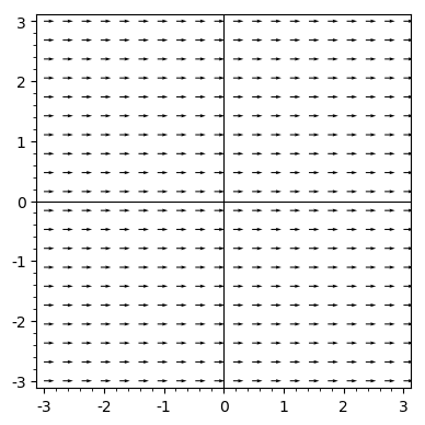
IMPORTANT NOTE: The figure above does not represent the actual vector field. The vector \(\langle 1,0\rangle\) has magnitude \(1\). If we observe the figure in Example 1, we can see that the vectors have the same magnitude, but their magnitude is not one. Most computer algebra systems rescale the vectors automatically for a better visualization.
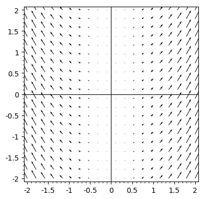
EXAMPLE 2. The figure below shows a visualization of the vector field \(\mathbf{F}(x,y)=\langle x, x^2\rangle\) in \(\mathbb{R}^2\).
Basic Operations
Curl
Suppose that \(\mathbf{F}(x,y,z) = F_1(x,y,z)\mathbf{i}+F_2(x,y,z)\mathbf{j}+F_3(x,y,z)\mathbf{k}\) is a vector field in \(\mathbb{R}^3\) and that the partial derivatives of \(F_1\), \(F_2\), and \(F_3\) all exist. Then, we define the curl of \(\mathbf{F}\) as
\[\text{curl } \mathbf{F} = \left(\frac{\partial F_{3}}{\partial y}-\frac{\partial F_{2}}{\partial z} \right)\mathbf{i}+\left(\frac{\partial F_{1}}{\partial z} - \frac{\partial F_{3}}{\partial x}\right)\mathbf{j}+\left(\frac{\partial F_{2}}{\partial x}-\frac{\partial F_{1}}{\partial y} \right)\mathbf{k}\]Another way to think of the curl is by using the “del” or nabla operator \(\nabla\) as a vector
\[\nabla = \mathbf{i}\frac{\partial}{\partial x} + \mathbf{j}\frac{\partial}{\partial y}+\mathbf{k}\frac{\partial}{\partial z}.\]Then we formally take the cross product of \(\nabla\) and \(\mathbf{F}\).
\[\begin{align*} \nabla \times \mathbf{F} =& \begin{vmatrix} \mathbf{i} & \mathbf{j} & \mathbf{k} \\ \frac{\partial}{\partial x} & \frac{\partial}{\partial y}&\frac{\partial}{\partial z}\\ F_1 & F_2 & F_3 \end{vmatrix} \\ =& \left(\frac{\partial F_{3}}{\partial y}-\frac{\partial F_{2}}{\partial z} \right)\mathbf{i}+\left(\frac{\partial F_{1}}{\partial z} - \frac{\partial F_{3}}{\partial x}\right)\mathbf{j}+\left(\frac{\partial F_{2}}{\partial x}-\frac{\partial F_{1}}{\partial y} \right)\mathbf{k} \\ =& \text{curl } \mathbf{F} \end{align*}\]Summarizing, we can think about the curl as
\[\text{curl }\mathbf{F} = \nabla \times \mathbf{F}\]EXAMPLE 3. We will calculate the curl of the vector field \(\mathbf{F} = 2xy\mathbf{i} -2xz\mathbf{j} + xyz\mathbf{k}\). We will use the cross product notation:
\[\begin{align*} \text{curl }\mathbf{F} = &\begin{vmatrix} \mathbf{i} & \mathbf{j} & \mathbf{k} \\ \frac{\partial}{\partial x} & \frac{\partial}{\partial y} & \frac{\partial}{\partial z} \\ 2xy & -2xz & xyz \end{vmatrix} \\ =& \left(xz + 2x \right)\mathbf{i} - \left(yz - 0 \right)\mathbf{j} + \left(-2z - 2x\right)\mathbf{k} \\ =& \left(xz + 2x \right)\mathbf{i} - yz \,\mathbf{j} -2(x + z)\mathbf{k} \end{align*}\]IMPORTANT REMARK. The curl of a vector field is a vector field.
Divergence
If \(\displaystyle\mathbf{F} = \langle F_1(x,y,z),F_2(x,y,z), F_3(x,y,z)\rangle\) is a vector field defined in \(\mathbf{R}^3\), the divergence of the vector field is defined as
\[\text{div } \mathbf{F} = \frac{\partial F_1}{\partial x} + \frac{\partial F_2}{\partial y}+ \frac{\partial F_3}{\partial z}\]assuming that all partial derivatives \(\displaystyle \frac{\partial F_i}{\partial x_i}\) exist for \(i=1,2,3\).
If the vector field is in \(\mathbb{R}^2\), then the divergence would be reduced to
\[\text{div } \mathbf{F} = \frac{\partial F_1}{\partial x} + \frac{\partial F_2}{\partial y}\]IMPORTANT NOTE. While the curl of t vector field is another vector field, the divergence of a vector field is a scalar field.
EXAMPLE 4. We will calculate the divergence of the vector fields
- \(\mathbf{F} = x^2y^2\,\mathbf{i} + e^{xy}\,\mathbf{j}\), which is \[ \text{div }\mathbf{F} = 2xy^2 + xe^{xy}.\]
- \(\mathbf{F} = xyz\,\mathbf{i} + \cos(yz)\,\mathbf{j} + z^3\,\mathbf{k}\), which is \[ \text{div }\mathbf{F} = yz-z\sin(yz) + 3z^2. \]
Similarly to what we did with the curl, we can use the nabla operator to give a formal way to compute the divergence by taking the dot product of the nabla operator and the vector field:
\[\nabla \cdot \mathbf{F} = \frac{\partial F_1}{\partial x} + \frac{\partial F_2}{\partial y}+ \frac{\partial F_3}{\partial z} = \text{div }\mathbf{F}\]So
\[\text{div }\mathbf{F} = \nabla \cdot \mathbf{F}\]